Part 4 - Modularize your application
Edit mePrepare for bringing in live streaming data by adding a test for unexpected data. You split the application into two modules that connect automatically at runtime by using exported streams. Then, you use additional dynamically connected modules from an existing Streams project to connect to the live data source and to display the moving vehicles on a map.
Watch this video for an overview.
Prerequisites
If you successfully completed the previous lab, skip to Step 1.
If you did not successfully complete the previous lab, you can continue with this lab by importing a Streams project that has been prepared for you and that contains the expected results from Part 3.
To import the Streams project:
- In the Project Explorer, right-click the current project (MyProject or MyProject1) and select Close Project. This gets it out of the way for builds or name conflicts without deleting any files.
- In the top Eclipse menu, click File > Import.
- In the Import dialog, click IBM Streams Studio > SPL Project. Then, click Next.
- Click Browse. In the file browser, expand My Home, scroll down, expand Labs, and select IntroLab. Click OK.
- Select MyProject2 and click Finish.
This starts a build, but you don't need to wait until it finishes. - In the Project Explorer, expand MyProject2 and then my.name.space.
- Double-click MyMainComposite to open it in the graphical editor.
- In the editor palette, right-click Toolkits. In the context menu, clear Show All Toolkits.
Add a test for unexpected data
A best practice is to validate the data that you receive from a feed. Data formats might not be well defined, ill-formed data can occur, and transmission noise can also appear. You do not want your application to fail when the data does not conform to its expectations. In this lab, you will be receiving live data.
As an example of this kind of validation, you will add an operator that
checks one attribute: the vehicle ID (id). In the data file all.cars,
all records have an id value of the form Cnnn (presumably, with "C"
for "car"). Even though it doesn't at the moment, assume that your
application depends on this format; for example, it could take a
different action depending on the type of vehicle indicated by that
first letter (say, "B" for "bus"). Also, there might be a system
requirement that all vehicle IDs must be exactly four characters.
Rather than silently dropping the tuple when it does not match requirements, it is better practice to save the "bad" data so that you can audit what happened and later perhaps enhance the application.
In summary, the vehicle ID (id attribute) specifications are as follows:
| Criterion | Value |
|---|---|
| First character | "C" |
| Length | 4 |
Therefore, if any data comes in with an unexpected value for id, your program will shunt it aside as invalid data. There are several operators that can take care of this. Which one you use is to some degree a matter of taste. You have already used one that works well, which is the Filter. So let's use a different one here.
The Split operator sends tuples to different output ports (or none) depending on the evaluation of an arbitrary expression. This expression can, but does not need to, involve attribute values from the incoming tuple. It can have as many output ports as you need. In this case, you need only two: one for the regular flow that you've been dealing with (the "valid" values), and one for the rest (the "not valid" ones).
The Split mechanism works as follows. (See the example in the figure below.)
- The N output ports are numbered 0, 1, …, N-1.
- A parameter called index contains an arbitrary expression that returns a 64-bit integer (an int64 or, if unsigned, a uint64).
- This expression is evaluated for each incoming tuple.
- The expression's value, n, determines which output port p the
tuple is submitted to:
- If n ≥ 0, p = n modulo N
- If n < 0, the tuple is dropped

Tip: At any time as you follow the steps below, use Layout and Fit to Content to keep the graph organized and visible.
- Add a Split operator to the graph. In this case, you need one with
two output ports.
- In the graphical editor, find the Split operator by using the Find box or browsing to Toolkits > spl > spl.utility > Split.
- Drag a Split operator (not a template) into the canvas and drop it directly onto the Throttled stream (output of the Throttled operator).
- Drag an Output Port from the palette (under Design) onto the Split operator. This gives it a second output port.
- Capture the Split's second output stream in a file:
- Add a FileSink to the graph.
- Drag a stream from the second output of the Split to the input of the new FileSink.
- Drag the LocationType schema from the palette (under Current
Graph/Schemas) onto the new stream. This turns it from a
dashed line into a solid line.
Notice that the new stream from the Split's first output port is already solid. It automatically inherits the schema from the original Throttled stream.
- Edit the properties of each of the new streams. In the General
tab, rename the first stream, which is the one that goes to
Filtered, to
Expected. Rename the second one toUnexpected. - Configure the Split operator. Because it has two output streams, it
is better to set a descriptive alias than to blank it out;
otherwise, it would be known by the name of the first output stream
(
Expected), which is misleading.- Edit the operator properties. In the General tab, rename it
to
IDChecker. - In the Param tab, click Add. Then, select index and click OK.
- In the Value field for the index parameter, enter the
following string exactly as shown. The "
l" after 0 and 1 is a lowercase letter L that indicates a "long" 64-bit integer:
substring(id,0,1) == "C" && length(id) == 4 ? 0l : 1l
This means that if the substring of the id attribute starting at offset zero with length one (in other words, the first character of id) is "C" and the length of the id attribute is four, then zero; otherwise one. Therefore, proper IDs go out from the first port (Expected), and everything else goes out from the second portUnexpected.
SPL expression language syntax: The syntax <Boolean-expression> ? <action-if-true> : <action-if-false> is known from C, Java, and other languages. The functions substring(string,start,length) and length(string) are from the Standard Toolkit. The suffix "l" (the lowercase letter L) indicates that the numbers are 64-bit values ("long" integers). SPL does not make implicit type conversions. Integer numbers with no suffix are 32-bit values and assigning one to a 64-bit parameter would result in an error.
- Edit the operator properties. In the General tab, rename it
to
- Configure the new FileSink operator. You've used a FileSink in two
previous sections, so refer to those if you forgot how to do it.
- Rename the FileSink operator to
ErrWriter. - Set the following parameter values:
- Rename the FileSink operator to
| Parameter | Value |
|---|---|
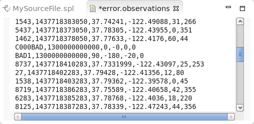
| file | "error.observations" |
| flush | 2u |
| format | csv |
| quoteStrings | false |
Flushing buffered file writes: FileSink performs buffered file I/O, meaning that it writes to buffers maintained by system libraries rather than directly to disk. These buffers are only written out to disk (flushed) as they fill up, or when the requesting application terminates. When the output is a slow trickle, this can mean that you will not see anything in the file for a long time. Setting flush to 2u (the u is for "unsigned" integer) guarantees that you will see data at least in batches of two records.
- Save, wait for the build to finish, launch the app, and verify that the original output files, filtered.cars and average.speeds, are being written to the data directory as before and that the new output file error.observations has at least two records in it after a suitable amount of time. The input file contains two records with a malformed ID.
Split off the ingest module
Now, it gets interesting. In a Streams application, data flows from operator to operator on streams, which are fast and flexible transport links. The Streams application developer is not concerned with how these are implemented. They might work differently between operators running on different hosts, in different PEs on the same host, or in the same PE, but the logic of the graph stays the same. An application requires explicit source and sink operators to exchange data with the outside world through file I/O, database connections, TCP ports, HTTP REST APIs, message queues, and so on.
However, for Streams applications that run in the same instance, another mode of data exchange is possible: Export and Import.
- An application exports a stream, making it available to other applications running in the instance.
- One or more applications can import such a stream based on flexible criteria.
- After exported streams are connected, they behave like all the other streams that run between PEs in an application, and they are fast and flexible. It's only at the time a job is submitted or canceled that the runtime services get involved to see which links need to be made or broken. After that's done, there is no performance impact.
But there is a tremendous gain in flexibility. Application stream connections can be made based on publish-and-subscribe criteria, and this allows developers to design completely modular solutions where one module can evolve and be replaced, removed, or replicated without affecting the other modules. It keeps individual modules small and specialized.
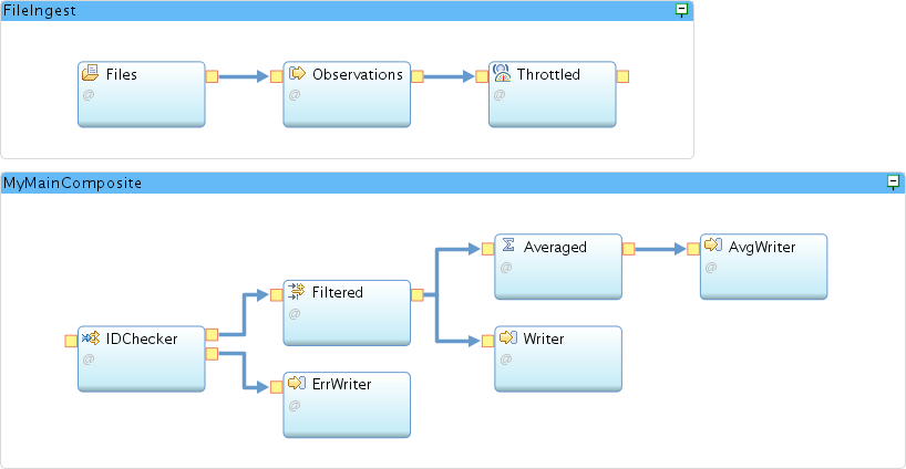
In this tutorial so far, you built a monolithic application, but there is a logical division. The front end of the application from DirectoryScan to Throttle reads data, in this case from files, and replays that data in a controlled fashion to make it look like a real-time feed.
The rest of the app from Split to FileSinks performs analysis and writes out the results. If you split off the front end into a separate Ingest module, you can imagine that it's easy to have another module alongside it or as a replacement that produces tuples that have the same structure and similar contents but that come from a completely different source. And that is exactly what this part of the tutorial will do: add another module that reads a live data feed and makes the data available for processing by the rest of this application.
In the graphical editor, drag a Composite (under Design in the
palette) and drop it on the canvas outside of any graphical object, not
on the existing main composite. The editor will call it Composite.
Rename it to FileIngest.
Notice that the new composite appears in the Project Explorer, but it
does not have a build associated with it.
Create a build for the new composite. In the Project Explorer, right-click the FileIngest main composite. Select New > Build Configuration. In the dialog, change the Configuration name to BuildConfig, accept all other defaults, and click OK.
Move the three front-end operators from the old main composite to the new:
In MyMainComposite, select the three operators Files, Observations, and Throttled. To do this, hold down the Ctrl key while you click each one. Cut them to the clipboard by pressing Ctrl+X or right-click and select Cut.
Select the FileIngest Paste the three operators in by pressing
Ctrl+V or right-click and select Paste.
You now have two applications (main composites) in the same code module
(SPL file). This is not standard practice, but it does work. However,
the applications are not complete: you have broken the link between
Throttled and IDChecker.
Set up the new application (FileIngest) for stream export:
- In the palette, find the Export operator and drop one (not a template) into the FileIngest
- Drag a stream from Throttled to the Export Note that the schema is remembered even when there was no stream because it belongs to the output port of Throttled.
- Edit the Export operator's properties. Rename it to FileExporter.
- In the Param tab, add the properties parameter. In the Value
field for properties, enter the following:
{ category = "vehicle positions", feed = "sample file" }
This action publishes the stream with a set of properties that are completely arbitrary pairs of names and values. The idea is that an importing application can look for streams that satisfy a certain subscription, which is a set of properties that need to match. - The FileIngest application builds, but MyMainComposite still has errors.
Set up the original application for stream import:
- In the palette, find the Import operator and drop it into the old main composite.
- Drag a stream from Import_11 to IDChecker.
- Assign a schema to this stream by dragging and dropping LocationType from the palette.
- Rename the new stream to Observations. There is already another stream called Observations, but it is now in a different main composite, so there is no name collision.
- Select the Import operator and rename it to Observations by blanking out the alias.
- In the Param tab, edit the value for the subscription parameter.
Replace the placeholder parameterValue with the following Boolean
expression:
category == "vehicle positions"
Notice that this is only looking for one property: the key category and the value "vehicle positions". You can ignore the other one that happens to be available, because if the subscription predicate is satisfied, the connection is made as long as the stream types match. - Save.
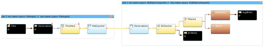
Test the new arrangement of the two collaborating applications.
- In the Instance Graph, minimize or hide any remaining jobs. Don't cancel them if you want to observe back-pressure later on. Set the color scheme to Flow Under 100 [nTuples/s]. Enlarge the view so you can easily see the two jobs.
- In the Project Explorer, launch the old application MyMainComposite.
- Launch the new application FileIngest.
Notice that the tuples flow from operator to operator throughout the instance graph even though the application is divided into two main composites. Leave the two applications running. You'll be adding two more.
Add a live feed
Rather than building a live-data ingest application from scratch, you will import a Streams project that has already been prepared. This application uses an operator called HTTPGetXMLContent to connect to a web services feed from NextBus.com and periodically (every 30 seconds) download the current locations, speeds, and headings of San Francisco Muni's buses and trams. That operator comes from a version of the com.ibm.streamsx.inet toolkit that is available only on GitHub. This toolkit was installed in your environment when you installed the tutorial files.
The application parses, filters, and transforms the NextBus.com data and makes the result look similar to the file data although some differences remain. It exports the resulting stream with a set of properties that match the subscription of your processing application. When you launch the NextBus application, the connection is automatically made and data flows continuously until you cancel the job.
To add a live feed:
- Before you can use the NextBus project, tell Studio where to find
the version of the com.ibm.streamsx.inet toolkit that it depends on:
- In the Streams Explorer, expand IBM Streams Installations [4.2.0.0] > IBM Streams 4.2.0.0 > Toolkit Locations.
- Right-click Toolkit Locations and select Add Toolkit Location.
- In the Add toolkit location dialog, click Directory and browse to My Home > Toolkits. (My Home is at the top; the dialog starts in the separate Root tree.) Select Toolkits and click OK.
- Click OK
If you expand the new location (Local) /home/streamsadmin/Toolkits, you see com.ibm.streamsx.inet[2.7.4]. This is different from the version of this toolkit that is installed with Streams (2.0.2), so the NextBus project can select the right one by version. The 2.0.2 version is under the location STREAMS_SPLPATH.
- Import the NextBus project:
- In the top Eclipse menu, click File > Import.
- In the Import dialog, click IBM Streams Studio > SPL Project. Then, click Next.
- Click Browse and in the file browser, expand My Home and select Toolkits. Click OK.
- Select NextBus and click Finish.
- Expand project NextBus and namespace ibm.streamslab.transportation.nextbus. Launch the application NextBusIngest. You might need to wait until the project build finishes.
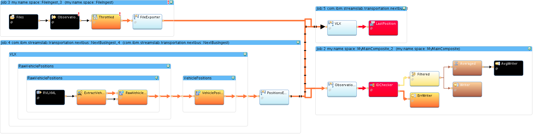
- Maximize and organize the Instance Graph. If you want, you can expand the nested composites in the NextBusIngest job.
- Check your results.
You should see the three applications that are connected. Tuples flow from the FileIngest job as long as you keep the "Infinite source" process running. Tuples flow from the NextBus job in 30-second bursts. The error.observations file gradually fills with records from NextBus. Their vehicle IDs do not conform to the "Cnnn" format.
Refresh the error.observations file periodically. To refresh the file, click in the editor showing the file and click Yes in the File Changed dialog, which appears when Studio detects that the underlying contents have changed.

Show location data on the map
The NextBus toolkit comes with another application that lets you view data in a way that is more natural for moving geographic locations, namely on a map. Similar to MyMainComposite, this application connects to the kind of stream exported by NextBusIngest and FileIngest. Without any further configuration, it can take the latitude and longitude values in the tuples and an ID attribute, and generate an appropriate map.
The map is simple and is intended only as a quick method for learning about your data.
- In the NextBus toolkit, launch NextBusVisualize. In the Edit
Configuration dialog, scroll down to the Submission Time Values.
Note the value of the port variable: 8080. Widen the Name column to
see the full name.
In the Instance Graph, each of the two exported streams is connected to each of the downstream jobs. The arrows look a bit confusing, but if you select each of the branches, you can untangle them.
 </img>
height=”400”}
</img>
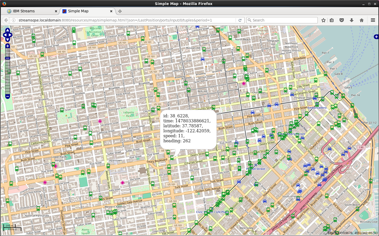
height=”400”} - To open the map in Firefox, double-click the Live Map desktop launcher. Minimize the Studio window or move it out of the way to see it. You will see a map of the San Francisco Bay Area with a large number of green bus markers crowding the city and blue cars concentrated in the downtown area.
- Use the map controls or mouse wheel to zoom in and pan (hold down
the left mouse button to drag and center the map) so that you can
see the individual vehicles. The buses jump around as their
locations are updated. You can see that the map is live!
The map refreshes every second, but remember that NextBus data is updated only every 30 seconds. If you zoom in far enough by clicking the zoom tool three times from the starting level, you can see the simulated cars from the file move continually around downtown San Francisco. They jump periodically, as the locations start over at the top of the file.
Click any one of the markers to get the full list of attributes for that vehicle.
 </img>
Optional_ Investigate back-pressure
This section builds on your exploration of the Streams Console in Part 3. It assumes that you have kept the job from Part 3 running for at least 40 minutes. To proceed, go back to the Application Dashboard in the Streams Console.
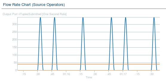
Because the file is read every 45 seconds and the throttled drawdown takes a little longer than that (47.55 s), the Throttle’s input buffer eventually fills up. If you let the job or jobs run long enough, a red square or yellow triangle will show in the PE Connection Congestion row of the Summary card. (The congestion metric for a stream tells you how full the destination buffer is, expressed as a percentage.) At the same time, the Flow Rate Chart shows more frequent, lower peaks: the bursts are now limited by the filling up of the Throttle’s input buffer instead of by the data available in the file.
- Hover over the information tool in the PE Connection Congestion
row in the Summary card to find out exactly which PEs are
congested and how badly.
Also, notice how the pattern in the Flow Rate Chart is now different compared to when the job was young.
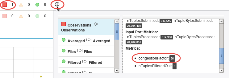
- View the information panel that shows Observations > Observations at the top of the list. This means that congestion is observed on a stream called Observations at the output port of an operator of the same name. (You did that by removing the operator alias.)
- Scroll down the right side of the panel to see the congestionFactor
metric, which is at the maximum value of 100. Note, however, that
while Observations is the one that suffers congestion, it is the
next operator named Throttled that causes it.
What will happen eventually if you let this run for a long time? Will the FileSource operator continue to read the entire file every 45 seconds? What happens to its input buffer on the port receiving the file names? How will the DirectoryScan operator respond?
These questions are intended to get you thinking about a phenomenon called back-pressure. This is an important concept in stream processing. As long as buffers can even out the peaks and valleys in tuple flow rates, everything will continue to run smoothly. But if buffers fill up and are never fully drained, the congestion moves to the front of the graph and something has to give. Unless you can control and slow down the source (as conveniently happens here), data will be lost, which cannot be avoided.
Summary
You should now understand how to add a test for unexpected data by splitting the application into two modules that connect automatically at runtime by using exported streams.
You should also know how to use additional dynamically connected modules from an existing Streams project to connect to the live data source and to display the moving vehicles on a map.