Part 3 - Apply enhanced analytics
Edit meIn this lab, you will enhance the app you've built by adding an operator to compute an average speed over every five observations, separately for each vehicle tracked. After that, you will use the Streams Console to monitor results.
So far, the operators you've used look at each tuple in isolation, and there was no need to keep any history. However, for many analytical processes, it is necessary to remember some history to compute the desired results. In stream computing, there is no such thing as "the entire data set," but it is possible to define buffers holding a limited sequence of consecutive tuples, for example, to compute the average over that limited subset of tuples of one or more numeric attributes. Such buffers are called windows. In this part, you will use an Aggregate operator to compute just such an average.
Watch this video for an overview.
Prerequisites
If you successfully completed the previous lab, skip this section and go to Step 1.
If you did not successfully complete the previous lab, you can continue with this lab by importing a Streams project that has been prepared for you and that contains the expected results from Part 2.
To import the Streams project:
- In the Project Explorer, right-click the current project (MyProject or MyProject1) and select Close Project. This gets it out of the way for builds or name conflicts without deleting any files.
- In the top Eclipse menu, click File > Import.
- In the Import dialog, click IBM Streams Studio > SPL Project. Then, click Next.
- Click Browse. In the file browser, expand My Home, scroll down, expand Labs, and select IntroLab. Click OK.
- Select MyProject2 and click Finish.
This starts a build, but you don't need to wait until it finishes. - In the Project Explorer, expand MyProject2 and then my.name.space.
- Double-click MyMainComposite to open it in the graphical editor.
- In the editor palette, right-click Toolkits. In the context menu, clear Show All Toolkits.
Add a window-based operator
You will compute average speeds over a window separately for vehicles C101 and C133. Use a tumbling window of a fixed number of tuples: each time the window collects the required number of tuples, the operator computes the result and submits an output tuple, discards the window contents, and is again ready to collect tuples in a now empty window.
Window partitioning based on a given attribute means that the operator will allocate a separate buffer for each value of that attribute—in effect, as if you had split the stream by attribute and applied a separate operator to each substream. The specifications are summarized in the following table:
| Specification | Value |
|---|---|
| Operator type | Aggregate |
| Window specification | Tumbling, based on tuple count, 5 tuples |
| Window partitioning | Yes, based on vehicle ID (id) |
| Stream to be aggregated | Filtered |
| Output schema | id rstring time int64 avgSpeed float64 |
| Aggregate computation | Average(speed) |
| Results destination | File: average.speed |
- Add the two required operators:
- In the graphical editor's palette filter box, enter
agg. Drag an Aggregate operator into the main composite. The editor calls it Aggregate_6. This is you main analytical operator. - In the palette filter, enter
filesink. Drag a FileSink into the main composite: FileSink_7. This will let you write the analytical results to a file.
- In the graphical editor's palette filter box, enter
- Fold the two new operators into the graph by connecting one existing
stream and adding another:
- Drag a stream from Filtered to Aggregate_6. This means Aggregate_6 is tapping into the same stream that Writer is already consuming, so the schema is already defined. This is indicated in the editor by a solid arrow.
- Drag another stream from Aggregate_6 to FileSink_7. This stream does not yet have a schema, so the arrow is dashed.
- Click Layout and Fit to Content.
- Rename the new stream and operators:
- Rename the stream to
Averaged. - Rename the Aggregate operator to
Averagedby blanking out its alias. - Rename the FileSink to
AvgWriter.
- Rename the stream to
- Give the Averaged stream (output of the Aggregate operator) its own
schema. In the Schema tab of the Properties view for the stream,
enter attribute names and types:
- In the first field under Name, enter
id. Press Tab. - Under Type, enter
rstring.Press Tab to go to the next name field. - Continue entering (and using Tab to jump to the next field) to enter the output schema attribute names and types listed in the table above.
- In the first field under Name, enter
- Tell the Aggregate operator what to do:
- Select the Averaged operator. In the Properties view, go to the
Window tab. A placeholder window specification is already
completed, but you need to change it slightly.
- Click Edit.
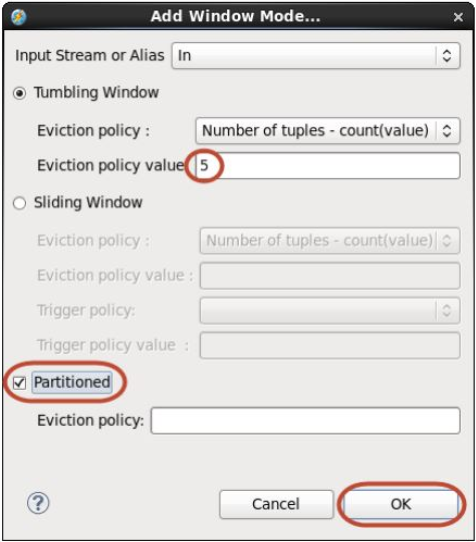
- In the Add Window Mode dialog, leave Tumbling Window selected.
- Set Eviction policy value to 5.
- Select Partitioned and leave Eviction policy blank.
- Click OK.
- Configure the window as partitioned on vehicle ID (the id
attribute).
- In the Param tab, click Add.
- In the Select parameters dialog, select partitionBy and click OK.
- In the partitionBy value field, enter
id.
- Specify the output assignment in the Output tab. You might
need to scroll down the list of tabs or make the Properties view
taller. Expand the twisty in front of Averaged in the Name
column. Widen the columns and enlarge the view horizontally to
see the full Name and Value columns. The attributes id and
time will be copied from the most recent input tuple. This
is already reflected in the Value column. By default, output
attribute values are assigned from attributes of the same name
based on the last input tuple.
Because the window is partitioned by id, all tuples in a window partition have the same value for this attribute. This is not the case for time, but in this example it is reasonable to use the most recent value.- Click Show Inputs. Expand the Filtered twisty and again LocationType. This shows the attributes that you can use to create an output assignment expression.
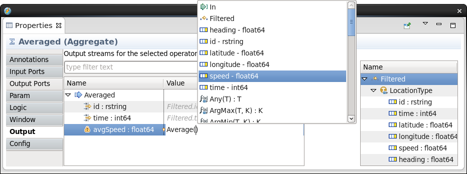
- Click in the value field for avgSpeed and press Ctrl+Space for content assist. In the list of possible entries, double-click Average(T) : T. (The syntax means that for any input type T, the output value will also be of type T.) This inserts Average(T) into the field.
- Again click in the value field for avgSpeed. Delete the
T inside the parentheses and keep the cursor there.
Press Ctrl+Space to show content assist, and this time
select speed - float64.
Tip for custom output functions: The functions shown in content assist are custom output functions specific to the Aggregate operator. They are not general-purpose SPL functions. Every output assignment must contain a call to one of these. The automatic assignments for the non-numeric attributes described above implicitly call the Last(T) custom output function.
- Select the Averaged operator. In the Properties view, go to the
Window tab. A placeholder window specification is already
completed, but you need to change it slightly.
- Specify where the results go. Select the newly added FileSink
operator (AvgWriter).
- In the Param tab, set the file parameter to
"average.speeds"(with the double quotation marks). - Click Add. In the Select parameters dialog, select
format and quoteStrings. Click OK. Set format to
csvand quoteStrings tofalse. - Save. Close the Properties view. Your application is ready to launch.
- In the Param tab, set the file parameter to
- Launch the application with a slight change to the configuration so
that each operator gets its own Processing Element (PE). This is in
preparation for your exploration of the Streams console.
- Right-click MyMainComposite in the Project Explorer and then select Launch > Launch Active Build Config To Running Instance.
- In Edit Configuration dialog, scroll down until you see the Fusion section.
- Change the Fusion scheme to Manual. Leave the Target number of PEs set to 10.
- Click Apply and then Launch.
Monitor the domain with the Streams Console
In this section, you will learn about the Streams Console, which is a general-purpose and web-based administration tool for IBM Streams. You will explore various parts of the Console, such as the application dashboard.
The Streams Console
The Streams Console is a web-based administration tool. Each Streams domain has its own console environment. The console interacts with one specific domain at a time based on its Streams Web Service (SWS) URL. In addition to managing and monitoring instances, resources, jobs, logging and tracing, and more, it serves as a simple data visualization tool. It is not intended to be a production-quality dashboard, but mainly a useful facility for monitoring applications and understanding data during development.
There are several ways to launch the Console: with a desktop launcher, or by looking up the URL and opening it directly in Firefox or any other browser from any machine with HTTPS access to the Streams environment. Normal user authentication and security apply. In this lab you open it from within Studio.
To open the Streams Console:
- In the Streams Explorer, expand Streams Domains. Right-click StreamsDomain (the only domain listed) and select Open Streams Console.
- In the Untrusted Connection page, expand I Understand the Risks and click Add Exception.
- If the Add Security Exception dialog appears, keep Permanently store this exception selected and click Confirm Security Exception.
- Log in as user
streamsadminwith the passwordpassw0rd.
The initial view is the Management Dashboard, which monitors the domain from an administrator's point of view. Each of the views, called cards, shows a specific type of object (PEs, jobs, instances, and so on) with a graphical view that lets you see at a glance what is going on.
The image shows a snapshot highlighting some of the graphically depicted information. For example, the PES card shows quickly which processing elements consume little memory and CPU (in the bottom left) and which consume a lot (top and right). This lets you identify quickly which operators to focus on during performance optimization or pinpoint a memory leak.
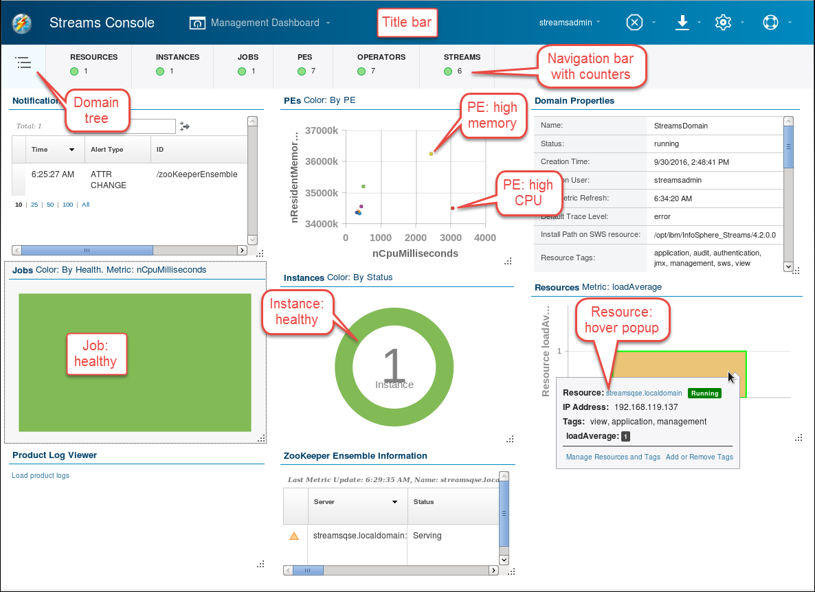
A PE or processing element is essentially a runtime process, which encapsulates one or more operators. Where the operator is the logical unit of operation, the PE is the unit of execution at runtime.
With only a single job running in a single instance on a single resource, many of the graphics are not very interesting, but they are useful when you are managing a real cluster with many running jobs. Hovering over the graphic in each card shows a panel with detailed information and links for drilling down further.
Also while hovering, controls appear in the top right of the card:
- Card Settings: color schemes, filters, and other settings appropriate for the information shown
- Refresh
- Card Flip Action: to show the tabular data behind a graphic
- Stack: minimize the card
- Max: maximize the card
Not all cards have all controls.
Explore the dashboard: resize, rearrange, and maximize cards. Flip a card (for example, PEs) to see the information in tabular form. Hover over one of the categories in the navigation bar and in the popup click Monitor [Instance | Job | …] to see a different set of cards.
Explore the Application Dashboard
Let's look more closely at your running application. While the Management Dashboard is designed for administrators, the Application Dashboard is more useful for developers. You can even set up your own dashboard by saving a set of cards in your preferred arrangement with a query to focus on just the jobs that are of interest to you.
- In the title bar, click Management Dashboard > Open
Dashboard > Application Dashboard.
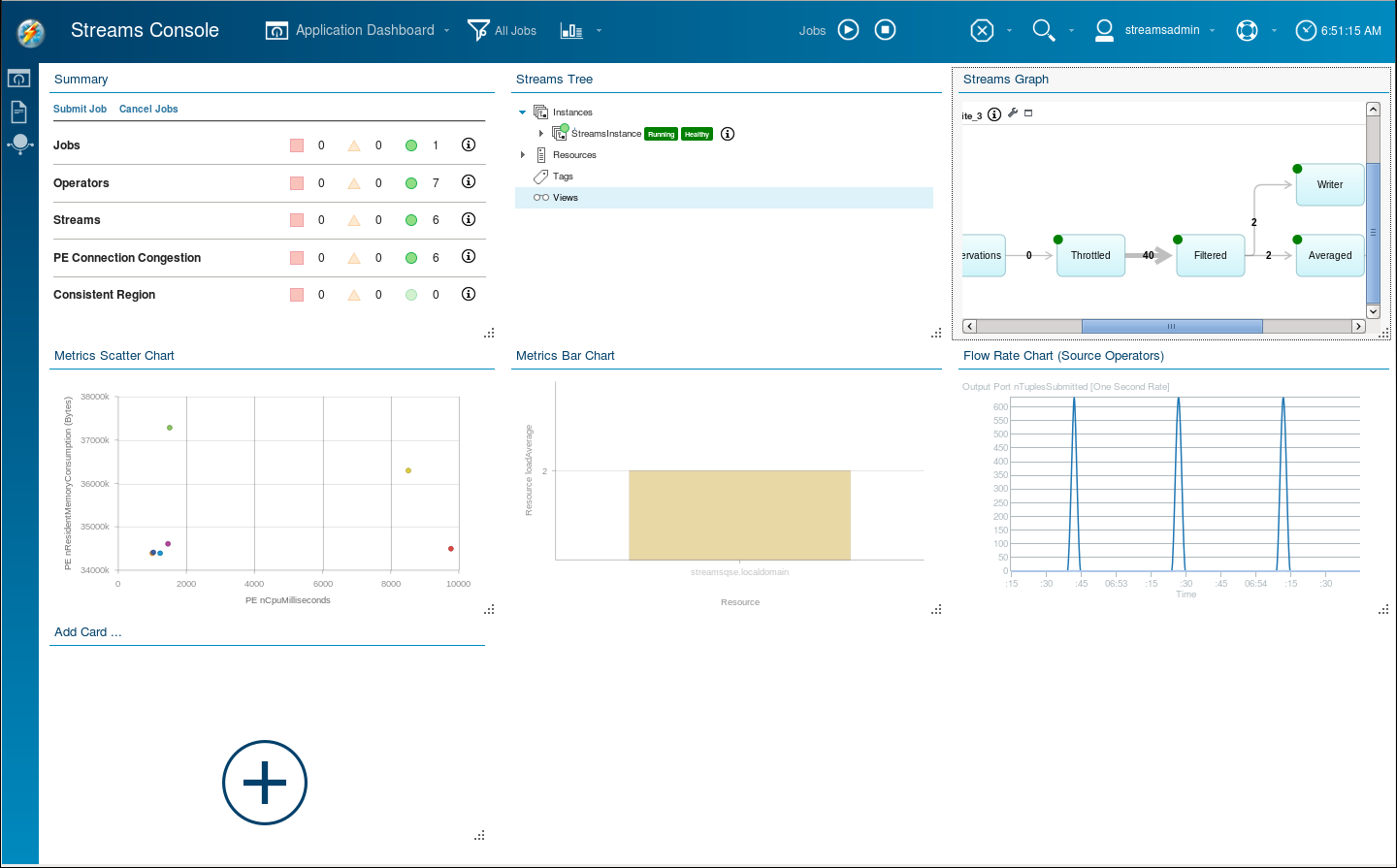
Some of the cards are equivalent to similar ones in the Management Dashboard:- Metrics Scatter Chart: shows the same information as PEs.
- Metrics Bar Chart: by default this shows the same information as Resources.
In addition, there are other cards with useful information:
- Summary card: shows at a glance the health or exception status of jobs, operators, streams, and congestion (and consistent regions, which this lab does not explore).
- Streams Tree: this is similar to the Streams Explorer in Studio.
- A Streams Graph: this is similar to the Instance Graph in Studio; if you have more than one job running, you must expand twisties to see their graphs.
- Flow Rate Chart: shows the tuple submission rates of all
source operators from all jobs.
The Flow Rate Chart is interesting. It shows sudden bursts of activity separated by periods of quiet. The source operator (FileSource, in this case) reads the file as fast as it can until it runs out of data. This fills the input port buffer of the Throttle, which slowly draws down that buffer at 40 tuples per second.
At just about the right time, when the Throttle operator is almost out of data, the same file is reported to the FileSource, which reads it again in one sharp burst. The chart shows the flow rate at zero most of the time with peaks up to just over 600 tuples per second spaced 45 seconds apart. Note that the chart shows a moving average over three seconds. In reality, the FileSource reads the entire file containing 1902 tuples in less than a second.
- Leave the job or jobs running.
Continue with the next lab. You will come back to the Console and your running job at the end of Part 4 to learn more about a concept called back-pressure, which is unique to stream processing.
Monitor jobs
- Maximize the Streams Graph card. You can also enlarge it by using the resize handle at the bottom right of the card. Enlarge it just enough to show the entire graph. Move it to another position and remove other cards as you see fit.
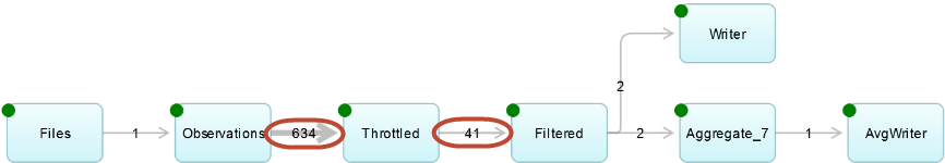
- Review the graph. The graph is familiar from the Instance Graph
in Studio, though it represents information in slightly different
ways. It labels every stream with the tuple rate, and indicates
operator health by a colored dot. As in the Instance Graph, relative
tuple rate sets the thickness of the arrow. Usually the
Throttled stream, at 40 tuples per second (give or take a few),
is the thickest, but every so often the Observations stream,
normally at zero, exceeds it. You observed the same behavior in the
Flow Rate Chart.
The Streams Graph is an alternative to the Summary card to detect trouble (unhealthy PEs) and to identify bottlenecks that can affect throughput performance. A bottleneck is an operator that limits the flow of tuples, usually because it cannot process any more tuples per second with the CPU cycles it has. If you do the optional section on back-pressure at the end of Part 4, you will see that the Throttle operator is the cause of congestion that builds up over time.
Summary
Now, you know how to enhance the application that you've built by adding an operator to compute an average speed over every five observations, separately for each vehicle tracked and how to monitor the results in the Streams Console.