Part 1 - Develop a simple application
Edit meIn this section, you will develop an application for a simple scenario: read vehicle location, speed, and other sensor data from a file, look for observations of a specific few vehicles, and write the selected observations to another file.
Watch this video for a summary of what we will cover.
Overview
The application will perform the following tasks:
- Read vehicle location data from a file
- Filter vehicle location data by vehicle ID
- Write the filtered vehicle location data to a file
You design the application graph in the graphical editor. You’ll use three operators. An operator is the basic building block of a Streams application graph.
Create a project
You're ready to start building your application. First, you'll create a Streams project, which is a collection of files in a directory tree in the Eclipse workspace, and then an application in that project.
The New SPL Application Project wizard takes care of a number of steps in one pass: it creates a project, a namespace, an SPL source file, and a main composite.
In Streams, a main composite is an application. Usually, each main composite lives in its own source file (of the same name), but this is not required. This section does not explore composite operators or what distinguishes a main composite from any other composite.
To create a project and a main composite:
- Click File > New > Project. Alternatively, right-click in the Project Explorer and select New > Project.
- In the New Project dialog, expand IBM Streams Studio, and select SPL Application Project.
- Click Next.
- In the New SPL Application Project wizard, enter the following
information:
- Project name:
MyProject - Namespace:
my.name.space - Main Composite Name:
MyMainComposite
- Project name:
- Click Next.
- On the SPL Project Configuration panel, change the Toolkit name
to
MyToolkit. - In the Dependencies field, clear Toolkit Locations.
- Click Finish. Project dependencies: In the Dependencies field you can signal that an application requires operators or other resources from one or more toolkits---a key aspect of the extensibility that makes Streams such a flexible and powerful platform. For now, you will use only building blocks from the built-in Standard Toolkit.
- Check your results.
You should see the following items in Streams Studio:
- The new project shows in the Project Explorer view on the left.
- The code module named MyMainComposite.spl opens in the graphical editor with an empty composite named MyMainComposite in the canvas.
Tip for adding space: If you want to give the editor more space, close the Outline view, and collapse the Layers and Color Schemes palettes. (This section does not use them.)
Review the project explorer
The Project Explorer shows both an object-based and a file-based view of all the projects in the workspace.
- In Project Explorer, note that you can expand and collapse
MyProject by clicking the twisty on the left.
The next level shows namespaces (only one, in this case), a dependencies entry, and resources (directories and files).
Below the namespace, my.name.space, are main composites. Other objects, such as types and functions, if you had any, appear there also. - Under my.name.space, see the main composite
MyMainComposite.
The next level shows build configurations. Here, there is only one build configuration, named BuildConfig, that is created by default. You can create multiple builds, for debug, different optimization levels and other variations. - Expand Resources.
The next level shows a number of directories and two XML files that contain descriptions of the current application or toolkit. (In Streams, toolkit and application are the same in terms of project organization and metadata.)
The only directory you will use in this section is the data directory. By default, build configurations in Streams Studio specify this as the root for any relative path names (paths that do not begin with a forward slash "/") for input and output data files.
Default data directory
Streams applications do not have a default data directory unless you explicitly set one in the build specification. Here, you are simply taking advantage of a feature of Streams Studio, which will provide that specification by default. It works because you have only a single host.
Because Streams is a distributed platform that does not require a shared file system, you need to be careful when you specify file paths. A process accessing a file must run on a host that can reach it. In general, this means specifying absolute paths and constraining where a particular process can run. Using relative paths and a default data directory makes the application less portable. Rather than separately define the schema (stream type) in the declaration of each stream, create a type first so that each stream can simply refer to that type. Keeping the type definition in one place eliminates code duplication, and improves consistency and maintainability.
Create a type named LocationType for the vehicle location data that
will be the main kind of tuple flowing through the application.
Use the following information to create the stream type:
| Name | Type | Comments |
|---|---|---|
| id | rstring | Vehicle ID (an rstring uses "raw" 8-bit characters) |
| time | int64 | Observation timestamp (milliseconds since 00:00:00 on January 1, 1970) |
| latitude | float64 | Latitude (degrees) |
| longitude | float64 | Longitude (degrees) |
| speed | float64 | Vehicle speed (km/h) |
| heading | float64 | Direction of travel (degrees, clockwise from north) |
To define a stream type:
- In the graphical editor, right-click anywhere on the canvas outside
the main composite (MyMainComposite), and click Edit.
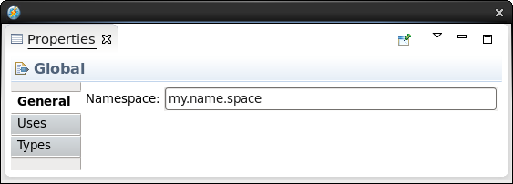
You see a Properties view, which floats above all the other views. Be sure that it looks the same as the following screen capture with the three tabs for General, Uses, and Types. If your Properties view does not look the same as the screen capture, dismiss the view and right-click again in the graphical editor outside the main composite.
- In the Properties view, click Types.
- Click Add New Type in the Name column.
- Enter
LocationType, and then press Enter. - Click Add Attribute below LocationType in the Name column,
and enter
id. - Press the Tab key to go to the Type column, and enter
rstring.
Tip for content assist: In the Type column, press Ctrl+Space to get a list of available types. Begin typing (for example, "r" forrstring) to narrow down the list. When the type you want is selected, press Enter to assign it to the field. This reduces keyboard effort and typing errors. - Press the Tab key to go to the next Name field.
- Enter the attribute names and types listed in the table above.
- Leave the Properties view open.
Tip for obscured views: The floating Properties view might obscure other views. An alternative is to use the Properties tab in the view at the bottom of the perspective. -
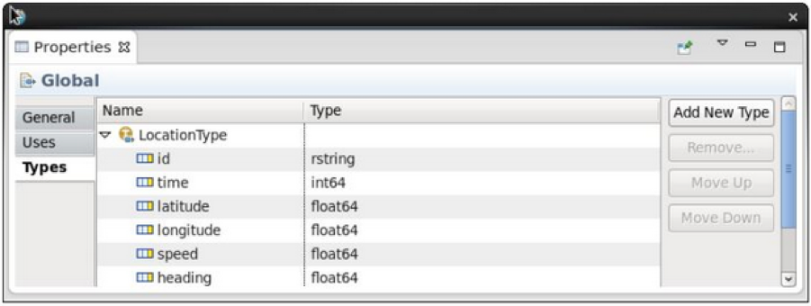
Check your results. The fields should look like the following screen capture:
 </img>
The tuple type LocationType is now available for you to use as a stream type in any main composite within the namespace my.name.space.
Create an application graph
You are now ready to construct the application graph and will need the following data for this section:
| Parameter | Value |
|---|---|
| Input file | /home/streamsadmin/data/all.cars |
| Output file | filtered.cars |
| File format | CSV (both input and output) Do not use quotation marks around strings on output |
| Filter condition | vehicle ID is "C101" or "C133" |
| Stream names | Observations (before filter) Filtered (after filter) |
With this information, you can create the entire application. You will use the graphical editor. There will be no SPL coding in this part of the tutorial.
Tip for seeing the code: If you want to see SPL code for what you are creating, right-click anywhere in the graphical editor and select Open with SPL Editor.
To drop the operators that you want into the graph, you need to find them in the palette, which is the panel to the left of the canvas.
Operator templates
Some operators appear once in the palette. Others (the ones you will use) have twisties and expand into one or more subentries. These are templates: invocations of the operator with specific settings, for example, a Filter operator with a second output port for rejected tuples. In this lab, the generic version (with the twisty) is always the correct one. Don't use the templates.
Operator names
The editor generates placeholder names for the operators that you drag onto the canvas. These placeholders include the operator type ("FileSink") and a sequence number ("1"). The sequence number depends on the order in which the operators are added to the graph, and yours might not match this document. You can safely ignore that. It does not affect anything in the application, and in any case, you will change the generated names later to match the role each operator plays.
Organize layout and maximize in view
To organize the layout, click the Layout button in the editor's toolbar. To zoom in and use all of the space in the graphical editor canvas, click the Fit to Content button. You can also use the slider in the toolbar to control the zoom level.
Before you add to the graph, reduce some clutter in the palette.
Initially, the list of toolkits is long because it shows all toolkits that Streams Studio knows about. The preconfigured tutorial workspace includes all toolkits installed with Streams. For now, you will not use any of those toolkits (and you have not declared any dependencies), so it is not helpful to have them in the palette.
- In the graphical editor, right-click Toolkits in the palette.
- In the context menu, clear Show All Toolkits.
- Find the following three operators:
- FileSource
- FileSink
- Filter
You can filter the palette contents and quickly get the ones you want.
Add operators to the application graph:
- In the graphical editor, go to the palette filter field, which shows
the word Find, and enter
fil. This narrows the palette down to a list that includes the three operators that you need.
Before you drop an operator: Make sure that the main composite MyMainComposite (and not one of the previously added operators) is highlighted when you drop the next operator. If a Confirm Overwrite dialog appears, click No and try again.
If you drop the operator on the canvas outside the main composite, the editor creates a new composite (called Comp_1) and places the operator inside. If that happens, undo the change (Ctrl+Z or click Edit > Undo Add Composite with Operator) and try again. - Select each operator with a twisty (one at a time) and drag it into the MyMainComposite main composite. Ensure that the green handles appear before you let go. The editor names the operators FileSink_1, FileSource_2, and Filter_3.
Add streams to your application graph
Output ports are shown as little yellow boxes on the right side of an operator. Input ports are on the left.
To create a stream, click an output port and start dragging. The cursor changes to a cross (+) as it drags a line from the output port. Release the mouse button as you drag, and then click the input port of another operator, which turns green when you hover over it, to complete the link. The two ports are now connected by a dashed line, which indicates that there is a stream, but its type is not yet defined.
- Add a stream connecting FileSource_2's output to Filter_3's input.
- Add another stream from Filter_3 to FileSink_1.
- Click Layout, then Fit to Content to organize the graph.
- Save your work (press Ctrl+S or the Save toolbar button,
or click File > Save).
Tip for hover popups: By default, hovering over an operator in the graphical editor invokes a popup that shows the SPL code behind that operator. As you build and lay out the graph, these popups might get in the way. Click the Toggle hover toolbar button to disable these popups. - Check your results.
You now have the complete graph, but none of the details have been specified.
The main composite and the three operators that it contains now have error indicators. This is expected because the code so far contains only placeholders for the parameters and stream types, and those placeholders are not valid entries.
Specify stream properties
The streams are what hold the graph together, so give meaning to them first. Tell the operators how to do their jobs later.
To assign a name and a type to a stream:
-
Select the stream (dashed arrow) connecting FileSource_2 and Filter_3. Sometimes you need to try a few times before the cursor catches the stream instead of selecting the enclosing main composite.
The Properties view, which you used earlier to create LocationType, now shows stream properties. Reposition and resize the view if necessary so that it doesn’t obscure the graph you’re editing. If you closed the Properties view, double-click the stream to reopen it.
- Enter descriptive stream names, which are preferable to the placeholder names generated by the editor, by clicking Rename in the Properties view (General tab).
-
In the Rename dialog, under Specify a new name, enter
Observationsand click OK.Notice that this saves the file and starts a build. This is because renaming an identifier is a form of refactoring, which means that not only the identifier itself but also any references to it must be found and updated. This requires a compilation step to ensure that the code is consistent and all references are known.
Specify the stream schema. You can do that in the Properties view, but because you already created a type for this, you can also drag and drop it in the graphical editor like any other object.
- In the graphical editor, clear the palette filter by clicking the
Eraser button next to where you entered
filThis makes all the objects visible again. - Under Current Graph, expand Schemas. This shows the LocationType type and the names of the two streams in the graph.
-
Select LocationType and drag it into the graph. Drop it onto the Observations stream, which is the one between FileSource_2 and Filter_3. Make sure that the stream’s selection handles turn green as you hover before you let go as shown below:
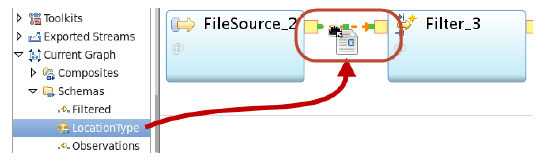 \
\If you open the Properties view to the Schema tab, it now shows a Type of LocationType and <extends> as a placeholder under Name. This indicates that the stream type does not contain some named attribute of type LocationType, but instead inherits the entire schema with its attribute names and types.
- Using the same drag and drop technique, assign the LocationType type to the other stream between Filter_3 and FileSink_1. Select that stream so that its properties show in the Properties view.
- In the Properties view, General tab, rename the stream to
Filtered.
Note: There is still an error indicator on FileSink_1 and because of that, on the main composite too. This is expected because you have not yet told the FileSink operator what file to write. You also need to provide details for the other operators.
Specify operator properties
With the streams fully defined, it is time to configure the operators.
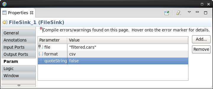
- In the graphical editor, select FileSink_1.
- In the Properties view, click the Param tab.
This shows one mandatory parameter, file, with a placeholder value ofparameterValue(not a valid value, hence the error marker). - Click on the field that says
parameterValue, and type"filtered.cars"(with the double quotes). - Press Enter.
Note that this is a relative path. It doesn't start with "/", so this file will go in the data subdirectory of the current project as specified by default for this application. - Click Add to add two more parameters.
- In the Select parameters dialog, select format and quoteStrings. You might need to scroll down to find it.
- Click OK.
- For the value of format, enter
csv. Do not use quotation marks; this is an enumerated value. - For the value of quoteString, enter
false. Do not use quotation marks; this is a Boolean value.
The properties view should look like this:
- The FileSource operator needs to know what file to read. In the graphical editor, select the FileSource_2 operator.
- In the Properties view (Param tab), click Add.
- In the Select parameters dialog, select file and format.
- Click OK.
- In the value for file, enter
"/home/streamsadmin/data/all.cars"(with quotes and exactly as shown—all lowercase). - For format, enter
csv. - You have to tell the Filter operator what to filter on. Without a
filter condition, it will simply copy every input tuple to the
output.
In the graphical editor, select Filter_3. - In the Properties view (Param tab), click Add.
- In the Select parameters dialog, select filter, and click OK.
- In the value field, enter the Boolean expression
id in ["C101","C133"]to indicate that only tuples for which that expression evaluates to true should be passed along to the output. (The expression with the key wordinfollowed by a list evaluates to true only if an element of the list matches the item on the left.) - Save your changes. The error markers disappear, and the application is valid.
- Make a few final changes.
Select the FileSink operator again. - Go back to the General tab in the Properties view.
- Rename the operator in the same way you renamed the two streams
earlier. Call it
Writer. - Select the FileSource operator, and rename it. This time, leave the name blank. Observe how the Identifier changes to Observations, which is the name of the output stream.
- Rename the Filter operator by removing the alias. In the graph, it will show as Filtered, which is the name of the output stream.
- Save your changes and dismiss the floating Properties view.
Tip for operator identifiers and aliases: SPL automatically assigns a name (identifier) to an operator by using the name of the output stream or streams. It also allows you to assign an alias to use as identifier instead, which gives you, as a developer, more control.
The graphical editor automatically assigns a generated alias to every operator, but in case of a single output stream, using the stream name is usually fine, so it is better to omit the alias. For an operator with multiple output streams, it's a good idea to provide a more descriptive alias. When there is no output stream (as for the FileSink) an alias is mandatory. - Check your results.
The Properties view might have been obscuring this, but each time you saved the graph, a build was started to compile the application. The progress messages are shown in the Console view (in a console called SPL Build). If you scroll back, you will see some builds that terminated on errors, with messages in red. (You might also want to maximize the Console view.) The last build should have completed without any errors.
Run your application
You are now ready to run this program or, in Streams Studio parlance, launch the build.
In the Project Explorer, right-click MyMainComposite. You might need to expand MyProject and my.name.space. Select Launch > Launch Active Build Config To Running Instance.
In the Edit Configuration dialog, click Apply, and then click
Launch.
You can set or change several options when you launch an application.
However, for now, ignore those options.
The Streams Launch progress dialog appears briefly. To see what
happened, switch consoles from the SPL Build to the Streams Studio
console.
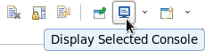
In the Console view, click the Display Selected Console button
on the right to switch consoles.
The Streams Studio console shows that job number 0 was submitted to the instance called StreamsInstance in the domain StreamsDomain.
Because nothing else seems to have happened, you need to look for some
result of what you've done. First, you'll view the job running in the
instance. Then, you'll inspect the results.
Switch to the Streams Explorer, which is the second tab in the view on the left, behind the Project Explorer.
Expand the StreamsDomains folder, and the Resources and
Instances folders under that.
The Resources folder refers to the machines that are available to the
domain. In this virtual machine, there is only one. Resource tags let
you dedicate different hosts to different purposes, such as running
runtime services or application processes. In this single-resource
environment, this is not relevant.\
Tip: For convenience, the Streams Jobs and Streams Instances folders
repeat information from the Instances folders under the listed domains,
but they lack further drill-down information.
You know that you have one instance StreamsInstance in the domain
StreamsDomain. The entry tells you that it is the default instance,
where launched applications will run unless otherwise specified, that it
is running and its current wall clock time. (You might need to widen the
view to see the status.)
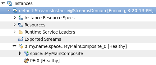
Expand default:StreamsInstance@StreamsDomain. This shows a number
of elements, but the only one you're interested in is the last one,
which is the job you have just submitted (a running application is
called a job):
0:my.name.space::MyMainComposite_0.
Its status should be Healthy. There is much information here about a job
and its constituent operators and Processing Elements (PEs), but you are
going to graphically explore it instead.
Tip for diagnosing problems: The most likely cause of an unhealthy
job is a mistake in the FileSource's file parameter, which isn't
caught by the compiler but can cause a "file not found" exception at
runtime. More elaborate debugging, such as using trace files and other
diagnostics, is beyond the scope of this lab.
 Right-click
default:StreamsInstance@StreamsDomain.
Right-click
default:StreamsInstance@StreamsDomain.
Select Show Instance Graph.
A new view opens in the bottom panel that shows a graph similar to that
in the graphical editor. However, this one shows in real time what is
running in the instance. If you launch multiple applications or multiple
copies of the same application, you will see them all. You can inspect
how data is flowing, see at a glance whether there are any runtime
problems, and monitor other metrics.
If necessary, expand or maximize the Instance Graph view. Click Fit to
Content in the view's toolbar.
There is a lot more to the Instance Graph, but you will explore it
further in the next lab.
Hover over Filtered to see current information about data flows and other metrics. Among other things, it will tell you that the input received 1902 tuples, and the output sent 95 tuples. This seems reasonable, given that the output should be only a subset of the input. But it also says that the current tuple rate on both input and output is 0/sec, so no data is currently flowing. Why? Because it has read all the data in the all.cars file, and there will never be any more data.
Inspect the results by looking at the input and output data.
Note that Streams jobs run forever. The input data is exhausted but the
job is still running. This is always true for a Streams application
running in an instance (distributed applications): a job can be canceled
only by manual (or scripted) intervention. In principle, a stream is
infinite even though in some cases, such as when reading a single file,
this might not be true.
In the top menu, click File > Open File.
In the Open File dialog, browse to streamsadmin/data/all.cars, and click OK. Studio opens the file in an editor view and shows location observations for multiple vehicle IDs: C127, C128, and so on.
In the Project Explorer (the first tab in the view on the left), expand Resources. There should be a file under data, but there is no twisty in front of the directory.
To update the view, right-click data, and select Refresh.
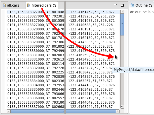
Expand the twisty and double-click filtered.cars. This file contains
coordinates, speeds, and headings only for vehicles C101 and C133.
Tip for showing files side by side: You can show two editors side by
side by dragging the tab of one of them to the right edge of the editor
view. As you drag, outlines appear, which arrange themselves side by
side as you approach the right edge. To undo this view, drag the tab
back to a position among the other tabs or close it.