Toolkit technical background overview

Edit me

The ElasticLoadBalance Operator

The ElasticLoadBalance operator, available on github under the streamsx.plumbing toolkit, is a drop-in replacement for the ThreadedSplit operator from the SPL Standard Library.

The new functionality is that it allows for runtime elasticity; in our context, runtime elasticity means that it will continually monitor its own tuple throughput, and adjust the active number of threads to seek out maximum performance.

To achieve this elasticity, I adapted our prior research work. Our papers Elastic Scaling of Data Parallel Operators in Stream Processing (IPDPS 2009) and Elastic Scaling for Data Stream Processing (TPDS 2014) present elasticity algorithms in the context of threads and processes distributed across hosts, respectively. The work in the paper from 2009 dynamically adapts the number of threads inside of a data-parallel operator, but it does not respond to workload changes. The paper from 2014 responds to workload changes, but it is designed to work across hosts, so it assumes larger communication costs. The ElasticLoadBalance operator incorporates lessons from both approaches to dynamically respond to workload changes in a threaded environment.

A note on the name: the ThreadedSplit operator that is currently part of the SPL Standard Toolkit already performs load balancing. As tuples arrive, it prefers to place tuples in the “next” buffer according to round-robin order. However, if that buffer is full, it will move on to the next available buffer, effectively load balancing the tuples across the output ports. LoadBalance is a more descriptive name for this operation, making this operator ElasticLoadBlance.

Why Use It?

The primary use-case for ElasticLoadBalance (and ThreadedSplit) is to enable taking advantage of data parallelism. In our context, data parallelism means invoking the same operator multiple times, and sending different tuples of the same stream to different invocations of that operator. Performance improves because we are processing tuples in parallel that previously were processed sequentially.

However, it is difficult to determine how much parallelism will yield the best performance. That is, is it best to invoke three parallel copies, or four? Currently, application developers must determine this by running their own experiments and manually varying the degree of parallelism. Developers must perform these experiments for every system they want to deploy their application to. Aside from the burden of taking extra time and effort, a major difficulty is that running such experiments on production systems is sometimes not an option. Further, such experiments may not answer how much parallelism is best under varying work loads.

Elasticity solves these problems by figuring out, at runtime, how much parallelism yields the best performance. Elastic solutions are robust to changes in both the hardware itself and the workload.

How It’s Used

The main difference when using the ElasticLoadBalance operator versus the ThreadedSplit operator is that you should over-provision the number of threads. Since there is one thread per output port, this means having more output ports than you think are required to achieve maximum performance on all deployments of the application. The number of output ports of the ElasticLoadBalance operator provides the upper-bound for the number of threads it can use. At runtime, it will dynamically determine exactly how many to use based on measured performance.

After installing the toolkit and pointing the SPL compiler to the toolkit itself, ElasticLoadBalance can be used as a drop-in replacement for the ThreadedSplit operator, such as in this example:

stream Src = Beacon() {}
(stream<Data> Src0;
 stream<Data> Src1;
 stream<Data> Src2;
 stream<Data> Src3;
 stream<Data> Src4;
 stream<Data> Src5) = com.ibm.streamsx.plumbing::ElasticLoadBalance(Src) {
    param bufferSize: 100u;
}
stream<Data> Res0 = Work(Src0) {}
stream<Data> Res1 = Work(Src1) {}
stream<Data> Res2 = Work(Src2) {}
stream<Data> Res3 = Work(Src3) {}
stream<Data> Res4 = Work(Src4) {}
stream<Data> Res5 = Work(Src5) {}

In this invocation of the ElasticLoadBalance operator, it has a total of six output ports, which means that it can use a maximum of six threads. Initially, it will start with only one active thread. After a period of time, it will measure the congestion and throughput it sees. It will then feed the observed throughput and congestion to its elasticity algorithm, which will make a recommendation for a new number of active output ports to use. This process (wait, measure, adapt) continues for the lifetime of the operator. Eventually, ElasticLoadBalance should settle on a number of threads that maximizes throughput. If the workload changes significantly, it will adapt.

How It Works

The operator periodically checks operator metrics for throughput, and the queue lengths for congestion. After measuring, it feeds the current values to its algorithms.

There are two basic principles behind the algorithm: providing evidence of performance improvement, and trusting data. Before increasing thread levels, we must have some evidence of a performance improvement trend. The improvement trend can come by looking at the current thread level and the level below it, or the current thread level and the level above it. If there is evidence of an increasing trend of performance as the thread level increases, then we should seek out a higher thread level to see if that also improves performance.

The notion of trust matters for adapting to changes in the workload. After taking a measurement at a particular level, we ?trust? that data. If we ever take a measurement that is significantly different from prior measurements at that level, then we un-trust all of the other data we have collected. After we un-trust our prior data, we are induced to re-explore thread levels we have already explored.

We achieve stability when we finally reach a thread level where we cease to see a performance improvement; we will settle on the level immediately prior to that point.

How It Performs

The following graphs show experiments using the performance tests included with the toolkit, under tests/performance. The stream graph is simple: a Custom operator generates tuples, and sends them to an ElasticLoadBalance operator. The ElasticLoadBalance operator has 32 output ports, which each go to a different invocation of a ?work? operator. The work operator performs a series of floating-point multiplies to simulate real work; the amount of multiplies depends on the tuple itself. Finally, all of the work operators send their result to a sink operator, which increments a counter.

Because the sink operator increments a counter, the upstream threads must grab a lock to protect the shared state. Grabbing this lock means that after a certain point (which depends on how expensive the tuples are to process), adding threads may harm performance. These experiments show that the ElasticLoadBalance operator is able to detect this performance degradation, and adapt.

Unless otherwise stated, all of these experiments were performed on a machine with 16 logical processors. As the ElasticLoadBalance operator has 32 output ports, it can potentially grow to use 32 total threads.

Expensive Tuples

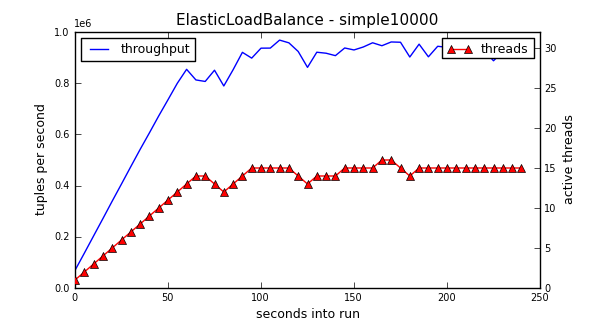
An “expensive” tuple in our context means that processing each tuple takes 10,000 floating-point multiplies. We can see that at the beginning of the run, as the number of threads continues to increase, so does the throughput. The number of threads eventually settles around 15. Again, note that this is a 16 logical processor machine, and that it could have used up to 32 threads. Rather, it discovered at runtime that about 15 threads yields the best performance, on this machine.

If we run this same experiment on a machine with less logical processors, the results are different, as shown in the following experiment.

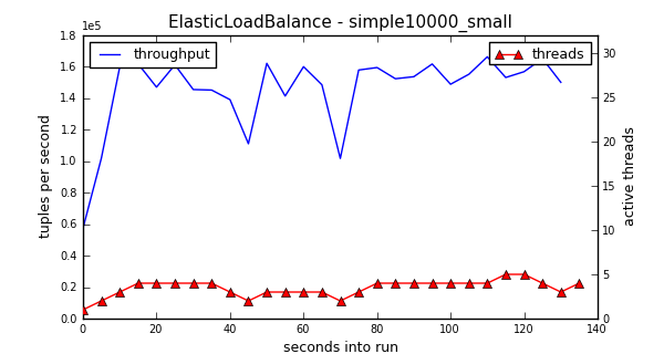
Medium Tuples

A “medium” tuple takes 1,000 floating-point multiplies to process each tuple. Unlike with the expensive tuples, the medium tuples do not saturate the hardware. With the expensive tuples, if we deployed that application to systems with more logical processors, it would probably grow to use more threads. But, in the medium case, it has access to more logical processors than it needs. The reason that it settles on about 8 threads, and not closer to 16, is that the cheaper costs of the tuples means that the threads spend more time contending on the lock in the downstream operator. Hence, more threads do not improve overall performance.

Cheap Tuples

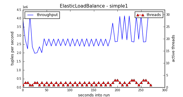
Finally, “cheap” tuples take only 1 floating-point multiply to process each tuple. We can see that despite having access to a total of 32 possible threads, the algorithm never explores higher than 3 threads.

Note that the oscillation in this experiment is rather high; that is, the thread level jumps frequently. The difficulty is that when work is so cheap, the execution time of a single tuple will necessarily be dominated by overhead. The overhead will be greatly affected by low-level system realities such as frequent lock contention, memory allocation and cache misses. Such occurrences are unpredictable, and will manifest in the throughput as significant noise.

The ElasticLoadBalance operator does have a parameter for dealing with noise, called throughputTolerance. The default value is 0.05, which means that throughput values within 5% of each other will be considered the same by the algorithm. Values closer to 1 for throughputTolerance will result in more stability, but the algorithm will also not come as close to the highest possible performance. Values closer to 0 for throughputTolerance will result in more oscillation, but the algorithm will find higher performance peaks. Because the cost to switching the thread level is so small (waking up a sleeping thread and updating some integers), I have made the default closer to 0.

Bursty Cost

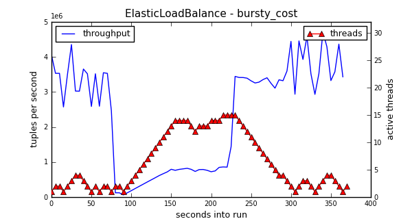
The previous experiments used a constant tuple rate and cost. The experiment above uses tuples with a variable cost. For the first 80 seconds, it sends cheap tuples. Until about 220 seconds, it sends expensive tuples, and then switches back to cheap tuples.

Note that when the tuple cost jumps to the expensive tuples at about 80 seconds, the throughput plummets because 1 or 2 threads is not enough to maintain high performance. But, it steadily climbs until the machine?s cores are saturated with work. When the experiment switches back to cheap tuples at about 220 seconds, the algorithm detects this change, and steadily puts threads to sleep.

Bursty Rate

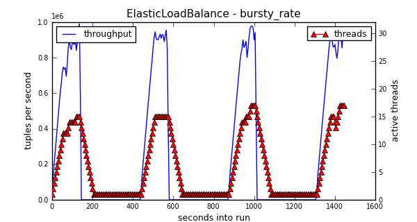
The other kind of burstiness is in arrival rate. That is, the previous experiment produced tuples as fast as it could, but changed how expensive they were. The experiment above maintains expensive tuples throughput the run, but it has long periods where it sends no tuples. We can see that as expected, the thread level increases when it starts receiving tuples, and decreases when no tuples are present. In this case, what causes the thread level to drop is the lack of congestion.

Conclusion

The ElasticLoadBalance operator is a drop-in replacement for the ThreadedSplit operator, and as demonstrated, it can adapt to different workloads and hardware.

Its purpose is to free developers from having to manually determine how much parallelism is best for their workload and hardware for each deployment. More examples of using the operator, and more details on its parameters, are available with the toolkit itself.